Google's Meridian: Getting Started with Modern Bayesian Marketing Mix Modelling

Many teams are testing Marketing Mix Modelling (MMM) internally right now, and some of that has been driven by the rise of Meridian from Google. Meridian is an open-source MMM framework developed by Google that offers a flexible, transparent, and well-documented workflow to accurately measure the incremental return on investment (ROI) of marketing channels.

Meridian uses a Bayesian MMM approach. This, in Linea’s opinion, is the gold standard for measuring incremental impact. The structure of Bayesian MMM allows marketers to best measure the uncertainty that exists in media campaigns and use external information to improve the accuracy of marketing decisions.

This article walks through a fully reproducible example using a simple dataset containing one revenue KPI and five media channels in a national-level model. The CSV file containing the data for this example is available here.

We will cover the 7 steps to running your open source Meridian Marketing Mix Modelling:

1. Installing Meridian
2. Importing packages and data
3. Specifying the model for Meridian
4. Running the model
5. Inspecting model quality
6. Exploring model results
7. Running a basic budget optimization

You can use this article to learn about Meridian without necessarily running the code, but if you do want to test Meridian yourself here are the requirements:

• Python: version 3.12 (or 3.11)
• A coding environment: I'll be using Jupyter

Installing Meridian

As mentioned above, you will need to be running Python version 3.12 or 3.11 as per the Meridian documentation. Then you can run the code below to install the Meridian package in your Python environment.

pip install google-meridian

This will install several other dependencies that will only work properly on the versions of Python specified above.

Importing packages and data

We start by importing the Meridian package into our coding environment.

# meridian functions
from meridian.data.data_frame_input_data_builder import DataFrameInputDataBuilder
from meridian.model.model import Meridian
from meridian.analysis import optimizer
from meridian.analysis import summarizer
from meridian.analysis import visualizer
from meridian.model import model
from meridian.model import prior_distribution as pdist, spec as specmod

# data manipulation
import pandas as pd

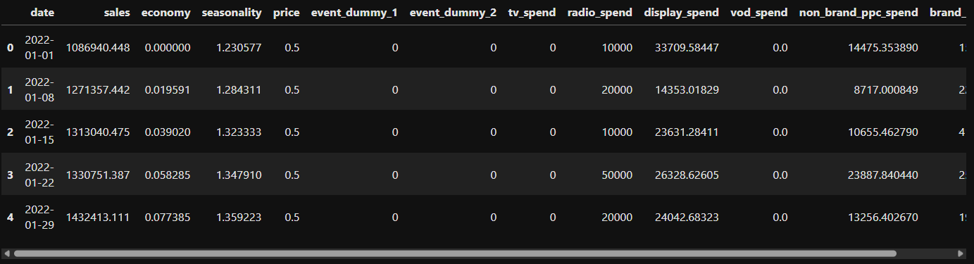
Then, using Pandas, we import our CSV file. This contains the breadth of variables that we are looking to test in our modelling.

df = pd.read_csv("./formatted_data_simple.csv")
df["date"] = pd.to_datetime(df["date"],format = "%d/%m/%Y")
df.head()

Specifying the model for Meridian

Now that we have our data, we can store the relevant variable names in the objects below, to specify:

• The dependent variable (kpi_name)
• The media variables (media_cols)
• The non-media variables (control_cols)

As a modeller, it is important at this point to ensure you have a wide breadth of control variables for model testing. When building a robust model, especially for an initial update, you will need to consider making variable transformations. For example, if you expect warm temperatures to impact the drivers of your ice-cream sales, then you could test:

• Average temperature
• Deviation from the average temperature vs. the historic average
• A threshold level (e.g. 25 degrees)

This is just an example of why expertise is still crucial when using tools like Meridian.

# all columns in the dataframe
all_cols = df.columns.tolist()

# the dependent variable
kpi_name = "sales"

# the media variables
media_cols = [
 'tv_spend',
 'radio_spend',
 'display_spend',
 'vod_spend',
 'non_brand_ppc_spend',
 'brand_ppc_spend']

# the control variables
exclude = set(media_cols + ["date", kpi_name])
control_cols = [c for c in all_cols if c not in exclude]

Then, using Meridian's DataFrameInputDataBuilder, we construct the model specification. This, input_data, is the object that stores the data that we will pass to the modelling function.

builder = DataFrameInputDataBuilder(kpi_type="revenue") \
    .with_kpi(df, kpi_col=kpi_name, time_col="date") \
    .with_media(
        df,
        media_cols=media_cols,
        media_spend_cols=media_cols,
        media_channels=media_cols,
        time_col="date"
    )\
    .with_non_media_treatments(
        df, 
        non_media_treatment_cols=control_cols, 
        time_col="date"
    )

input_data = builder.build()
model_spec = specmod.ModelSpec(
    knots=1,   # single coefficient over time -> constant baseline
)

Meridian's model specification does allow for some complexity to be added to the model (e.g. priors and different prior distributions). One critical aspect that is lacking in Meridian's, and most approaches available, is handling synergies. properly (i.e. will my marketing perform as well in periods with lower demand?). At Linea we developed an approach that not only tests synergies, but also measures the how much these synergies impact each variable.

Running the model

Using the input_data object, we can now instantiate the Meridian model. This creates a Bayesian MMM object that holds the model structure, priors and data. The next step is to run prior sampling to verify that the priors behave sensibly, followed by posterior sampling where the actual inference happens.

mmm = Meridian(input_data=input_data)
mmm.sample_prior(500)
mmm.sample_posterior(
    n_chains=2, n_adapt=2000, n_burnin=500, n_keep=1000, seed=0
)

For the purpose of this article we are using lightweight settings to keep computation fast enough for a tutorial. When running models in production, you will usually want to increase the number of chains, warmup period and kept samples to improve stability and convergence.

In our experience, we find that those running Bayesian models struggle with the time taken to run. For example, the default Meridian MMM model from the official documentation can take upto 1 hour to run. Other Bayesian modellers have suggested that they leave it to run overnight. This need not be the case. If you want Linea to speed up your Bayesian MMM model then arrange a call.

# mmm.sample_posterior(
#     n_chains=4,
#     n_adapt=4000,
#     n_burnin=1000,
#     n_keep=2000,
#     seed=0,
# )

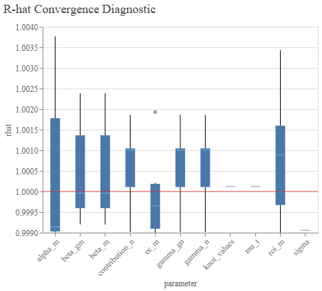
Inspecting model quality

Before looking at the results, it is good practice to examine diagnostics to confirm that the model converged properly. Meridian provides several built in tools for inspecting chain behaviour. Below we plot the R hat distribution, which is a common MCMC diagnostic indicating whether chains converged toward the same region of the posterior.

model_diagnostics = visualizer.ModelDiagnostics(mmm)
model_diagnostics.plot_rhat_boxplot()

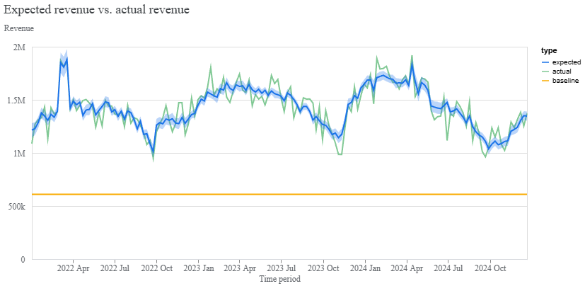
Once the sampler has converged, we can look at the overall fit of the model. The plot below compares observed data with modelled predictions across time, helping identify underfitting, overfitting and systematic deviations.

model_fit = visualizer.ModelFit(mmm)
model_fit.plot_model_fit()

Exploring model results

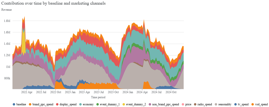
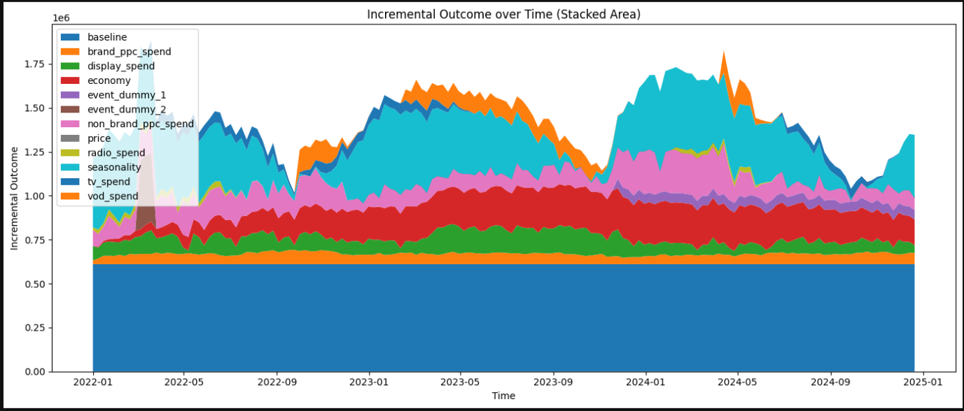
After confirming model quality, we can explore what the model learned about channel contributions. The following chart breaks down incremental impact over time, showing how each media input contributes to the outcome.

media_summary = visualizer.MediaSummary(mmm)
media_summary.plot_channel_contribution_area_chart()

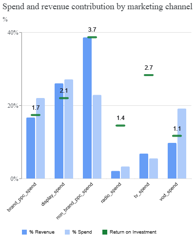
Another useful view compares spend with contribution, helping identify whether channels are delivering value relative to their cost. This plot can highlight under-invested or over-invested channels.

media_summary.plot_spend_vs_contribution()

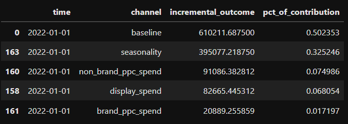
You can also access the contribution of each variable, using the media_summary object, to dive deeper into your model's results.

contrib = media_summary.contribution_metrics(
    include_non_paid=True,
    aggregate_times=False
)
contrib.head()

Running a basic budget optimization

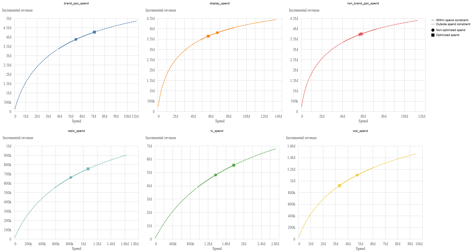
With estimated diminishing returns and channel response curves available, we can run a basic optimisation analysis. The optimizer searches for a better allocation of spend based on expected outcomes. Here we use the default configuration, which reallocates the historical budget to maximise performance.

budget_optimizer = optimizer.BudgetOptimizer(mmm)
optimization_results = budget_optimizer.optimize()
optimization_results.plot_response_curves()

This produces a set of recommended allocations and visual response curves, offering a first pass at how budget could be redistributed according to the model.

At Linea, we have found that the Meridian optimisation solution lacks the flexibility to run what-if scenarios. Also, as a code-based interface, it’s not a tool that Marketing teams or media agencies can easily use. That’s why we built the Linea Scenario Tool. It plugs into your Meridian MMM and offers an intuitive user interface for cross-channel allocation and campaign planning. Crucially, it allows you to overlay how future factors such as media cost inflation, economic impacts, or market changes will impact your cross-channel budget decisions. Test it with a free trial here.

The Meridian library is a useful option for teams that need a clear, technically robust MMM without relying on extensive internal tooling. It works well for organisations early in their analytics journey or those looking for a quick topline view of performance.

As modelling needs grow, though, generic frameworks reach their limits. Bespoke structures will deliver stronger accuracy and flexibility, especially when industry specifics and real world dynamics matter.

Linea provides custom MMMs built for each sector, incorporating features such as variable synergies, scenario and optimised scenarios that generate complete media plans. If you’re looking to move from a basic overview to a model that can support confident, detailed decision making, we’re here to help.